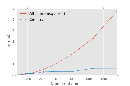
One of the conclusions from last post is a need for better profiling tools to show where time is spent in the code. Profiling Python + JIT'ed code requires dealing with a couple of issues.

The first issue is collecting stack information at different language levels. A native profiler collects a stack for the JIT'ed (or compiled extension) code, but eventually the stack enters the implementation of the Python interpreter loop. Unless we are trying to optimized the interpreter loop, this is not useful. We would rather know what Python code is being executed. Python profilers can collect the stack at the Python level, but can't collect native code stacks.

The PyPy developers created a solution in vmprof. It walks the stack like a native profiler, but also hooks the Python interpreter so that it can collect the Python code's file, function, and line number. This solution is general to any type of compiled extension (C extensions, Cython, Numba, etc.) Read the section in the vmprof docs on Why a new profiler? for more information.

The second issue is particular to JIT'ed code - resolving symbol information after the run. For low overhead, native profilers collect a minimum of information at runtime (usually the Instruction Pointer (IP) address at each stack level). These IP addresses need to resolved to symbol information after collection. Normally this information is kept in debug sections that are generated at compile time. However, with JIT compilation, the functions and their address mappings are generated at runtime.

LLVM includes an interface to get symbol information at runtime. The simplest way to keep it for use after the run is to follow the Linux perf standard (documented here), which stores the address, size, and function name in a file /tmp/perf-<pid>.map.

To enable Numba with vmprof, I've created a version of llvmlite that is amenable to stack collection, at the perf branch here.

This does two things:

1. Keep the frame pointer in JIT'ed code, so a backtrace can be taken.¹
2. Output a perf-compatible JIT map file (not on by default - need to call enable_jit_events to turn it on)

To use this, modify Numba to enable JIT events and frame pointers:

1. In targets\codegen.py, at the end of the _init method of BaseCPUCodegen, add self._engine.enable_jit_events()
2. And for good measure, turn on frame pointers for Numba code as well (set CFLAGS=-fno-omit-frame-pointer before building it)

The next piece is a modified version of vmprof ( in branch numba ). So far all it does is read the perf compatible output and dump raw stacks. Filtering and aggregating Numba stacks remains to be done (meaning neither the CLI nor the GUI display work yet).

How to use what works, so far:

1. Run vmprof, using perf-enabled Numba above: python -m vmprof -o vmprof.out <target python>
2. Copy map file /tmp/perf-<pid>.map to some directory. I usually copy vmprof.out to something like vmprof-<pid>.out to remember which files correlate.
3. View raw stacks with vmprofdump vmprof-<pid>.out --perf perf-<pid>.map.

A previous post showed some performance improvements with the nsquared version of the code. This post will tackle the cell version of the code. In the nsquared version the time-consuming inner loop had no function calls. The cell version does call other functions, which may complicate optimization.

Times are all in μs/atom. System size is 4000 atoms. Hardware is Xeon E5-2630 v3 @ 2.4 Ghz, OS is Ubuntu 12.04.
The 'Initial Time' column results from the minimal amount of code changes to get the compiler working.
The 'Final Time' is the time after the tuning in this post.

Julia

The cell version contains the same issue with array operations as the nsquared version - the computation of dd allocates a temporary to hold the results every time through the loop.

The Devectorize package can automatically convert array notation to a loop. If we add the @devec annotation, the time drops to 43 μs/atom. Unfortunately, the allocation to hold the result must still be performed, and it remains inside the inner particle loop. If we manually create the loop and hoist the allocation out of the loop, time is 27 μs/atom.

The code uses dot to compute the vector norm. This calls a routine (julia_dot) to perform the dot product. For long vectors calling an optimized linear algebra routine is beneficial, but for a vector of length 3 this adds overhead. Replacing dot with the equivalent loop reduces the time to 23 μs/atom.

Looking through the memory allocation output (--track-allocation=user) shows some vector operations when the force array is zeroed and accumulated. Also in putAtomInBox in linkcell.jl. These spots are also visible in the profile output, but the profile output is less convenient because it is not shown with source. The @devec macro does work here, and the performance is now 7.7 μs/atom. Explicit loops give a slightly better time of 7.3 μs/atom.

Profiling shows even more opportunities for devectorization in advanceVelocity and advancePosition in simflat.jl Time is now 6.4 μs/atom.

The Julia executable has a -O switch for more time-intensive optimizations (it adds more LLVM optimization passes). This improves the time to 6.2 μs/atom.

The @fastmath macro improves the time a little more, to 6.1 μs/atom. The @inbounds macro to skip the bounds checks did not seem to improve the time.

The final Julia time is now within a factor of 3 of the C time. The code is here. It's not clear where the remaining time overhead comes from.

PyPy

The PyPy approach to JIT compilation is very general, but that also makes it difficult to target what code changes might improve performance. The Jitviewer tool is nice, but not helpful at a cursory glance. The vmprof profiler solves an important problem by collecting the native code stack plus the python stack. In this particular case, it reports at the function level, and the bulk of the time was spent in computeForce. I hope to write more about vmprof in a future post, as it could help with integrated profiling of Python + native code (either compiled or JIT-ed).

Cython

The simplest step is to add an initialization line and move some .py files to .pyx files. This gives 729 μs/atom. Adding types to the computeForce function and assigning a few attribute lookups to local variables so the types can be assigned (playing a game of 'remove the yellow' in the Cython annotation output) gives 30 μs/atom.

Adding types and removing bounds checks more routines (in halo.py, linkcell.py, simflat.py) gives 13 μs/atom.

Code is here. Further progress needs deeper investigation with profiling tools.

Numba

Starting with adding @numba.jit decorators to computeForce, and the functions it calls gives the initial time of 867 μs/atom. Extracting all the attribute lookups (including the function call to getNeighborBoxes) gives 722 μs/atom.

We should ensure the call to getNeighborBoxes is properly JIT-ed. Unfortunately, this requires more involved code restructuring. Functions need to be split into a wrapper that performs any needed attribute lookups, and an inner function that gets JIT-ed. Loop lifting automatically performs this transformation on functions with loops. On functions without loops, however, it needs to be done manually. Once this is done, the time improves dramatically to 47 μs/atom.

Hopefully the upcoming "JIT Classes" feature will make this easier, and require less code restructuring.

Code is here

Summary

Julia is leading in terms of getting the best performance on this example. Many of these projects are rapidly improving, so this is just a snapshot at their current state.

All these projects need better profiling tools to show the user where code is slow and to give feedback on why the code is slow. The Cython annotated output is probably the the best - it highlights which lines need attention. However it is not integrated with profiler output, so in a project of any size, it's not clear where a user should spend time adding types.

Julia has some useful collection and feedback tools, but they would be much more helpful if combined. The memory allocation output is bytes allocated. It's useful for finding allocations where none were expected, or for allocations in known hot loops, but it's less clear which other allocations are impacting performance. Ideally this could be integrated with profiler output and weighted by time spent to show which allocations are actually affecting execution time.

The term 'vectorize' as used by programmers has at least two separate uses. Both uses can have implications for performance, which sometimes leads to confusion.

One meaning refers to a language syntax to express operations on multiple values - typically an entire array, or a slice of a array. This can be a very convenient notation for expressing algorithms.

Here is a simple example (in Julia) using loop-oriented (devectorized) notation

a = ones(Float64, 10)
b = ones(Float64, 10)
# allocate space for result
c = zeros(Float64, 10)

for i in 1:10
    c[i] = a[i] + b[i]
end

Now compare with using vectorized (array) notation

a = ones(Float64, 10)
b = ones(Float64, 10)

# space for result automatically allocated

c = a + b

The vectorized notation is more compact. Julia and Python/Numpy programmers usually mean this when referring to 'vectorization'. See more in the Wikipedia entry on Array programming

John Myles White wrote a post discussing the performance implications of vectorized and devectorized code in Julia and R. Note that Python/Numpy operates similar to R as described in the post - good performance usually requires appropriately vectorized code, because that skips the interpreter and calls higher performing C routines underneath.

The other meaning of 'vectorization' refers to generating assembly code to make effective use of fine-grained parallelism in hardware SIMD units. This is what Fortran or C/C++ programmers (and their compilers) mean by 'vectorization'. In Julia, the @simd macro gives hints to the compiler that a given loop can be vectorized.

See more in the Wikipedia entry on Automatic vectorization

In previous posts, we've seen that adding type information can help the performance of the code generated by dynamic language compilers. The documentation for Cython annotations talks of 'Python interaction', and Numba has 'object' mode and 'nopython' modes. In post I will look more at what these mean, and how they affect performance.

To start, consider how values are represented in a computer, such as a simple integer ('int' type in C). The bare value takes 4 bytes in memory, and no additional information about it is stored, such as its type or how much space it occupies. This information is all implicit at run time ¹. That it takes 4-bytes and is interpreted as an integer is determined at compile time.

In dynamic languages, this extra information can be queried at run-time. For example:

>>> a = 10
>>> type(a)
<type 'int'>

The value stored in a has type int, Python's integer type. This extra information must be stored somewhere, and languages often solve this by wrapping the bare value in an object. This is usually called 'boxing'. The value plus type information (and any other information) is called a 'boxed type'. The bare value is called an 'unboxed type' or a 'primitive value'.

In Java, different types can be explicitly created (int vs. Integer), and the programmer needs to know the differences and tradeoffs. (See this Stack Overflow question for more about boxed and primitive types.)

Python only has boxed values ('everything is an object'). From the interpreter, this means we can always determine the type of a value. If we look a layer down, as would be needed to integrate with C, these values are accessed through the Python API. The base type of any object is PyObject. For our simple example, integers are stored as PyIntObject.

For example, consider the following Python code.

  def add():
    a = 1
    b = 1
    return a + b

One way to see what calls the interpreter would make is to compile with Cython. The following C is the result (simplified - reference counting pieces to the Python API are omitted.)

PyObject *add()
{
  PyObject *pyx_int_1 = PyInt_FromLong(1);
  PyObject *pyx_int_2 = PyInt_FromLong(2);
  PyObject *pyx_tmp = PyNumber_Add(pyx_int_1, pyx_int_2);
  return pyx_tmp;
}

Without type information, Cython basically unrolls the interpreter loop, and makes a sequence of Python API calls. The HTML annotation output highlights lines with Python interaction, and can be expanded to show the generated code. This gives feedback on where and what types need to be added to avoid the Python API calls.

Add some Cython annotations and the example becomes

 cdef int add():
    cdef int a
    cdef int b
    a = 1
    b = 1
    return a + b

Now the following code is generated

 int add()
 {
  int a = 1;
  int b = 2;
  return a+b;
 }

The add of the two integers is done directly (and runs much faster), rather than going through the Python API call.

Numba

If its type information is insufficient, Numba will call the Python API for every operation. Since all the operations occur on Python objects, this is called 'object' mode (slow). With sufficient type information, code can be generated with no calls to the Python API, and hence the name 'nopython' mode (fast).

Julia

Julia has boxed object types, but is designed to try use the unboxed types as much as possible. The most generic type is called 'Any', and it is possible to produce Julia code that runs this mode.
See the section on Embedding Julia in the documentation for more about Julia objects.

Julia's type inference only happens inside functions. This is why composite types (structures) need type annotations for good performance.

This example demonstrates the issue

type Example
    val
end

function add(a, b)
    return a.val + b.val
end

v1 = Example(1)
v2 = Example(2)

@code_llvm add(v1, v2)  # The @code_llvm macro prints the LLVM IR.  
t = add(v1, v2)
println("res = ",t)

Since the type of the 'val' element is not known, the code operates on a generic object type jl_value_t and eventually calls jl_apply_generic, which looks up the right method and dispatches to it at execution time. (The LLVM IR is not shown here - run the example to see it.) Doing all this at execution time is slow.

Now add the type annotation

type Example
    val::Int
end

The resulting LLVM IR (also not shown here) is much shorter in that it adds two integers directly and returns the result as an integer. With type information, the lookup and dispatch decisions can be made at compile time.

Note that Julia uses a Just In Time (JIT) compiler, which means compilation occurs at run time. The run time can be split into various phases, which include compilation and execution of the resulting code.

Summary

Hopefully this post sheds some light on how type information can affect the performance of dynamic languages.

The previous post introduced the CoMD miniapp in Python and Julia. This post will look a little deeper into the performance of Julia and various Python compilers. I will use the nsquared version of the code for simplicity.

The computeForce function in ljforce takes almost all the time, and it is here we should focus. In the nsquared version there are no further function calls inside this loop, which should make it easier to analyze and improve the performance.

The summary performance table (all times are in microseconds/atom, the system is the smallest size at 256 atoms)

(This table uses a different code version and different hardware, so the numbers are not comparable to the previous post)
(Hardware is i7-3720QM @ 2.6 Ghz and OS is Ubuntu 14.04)
The 'Initial Time' column results from the minimal amount of code changes to get the compiler working.
The 'Final Time' is the time after doing some tuning (for this post, anyway - there's still more work to be done).

HOPE

The HOPE compiler will compile the nsquared version, provided the branch involving the cutoff is modified to avoid the continue statement. The loop that zeros the force also needs a simple name change to the loop variable. The backend C++ compiler is gcc 4.8.4. No attempt was made to try different compilers or further optimize the generated code.

Numba

To use Numba, we need to add import numba to ljforce.py and add the @numba.jit decorator to the computeForce method. This gives the time in the initial column (450 μs/atom) , which is about a 20% improvement over the plain Python version.

Code involving attribute lookups cannot currently be compiled to efficient code, and these lookups occur inside this inner loop. And the compiler will not hoist attribute lookups outside the loop. This can be done manually by assigning the attribute to a temporary variable before the loop, and replacing the values in the loop body. This transformation enables effective compilation of the loop.

(Internally Numba performs loop-lifting, where it extracts the loop to a separate function in order to compile the loop.)

The beginning of the function now looks like

    @numba.jit
    def computeForce(self, atoms, sim):
        # hoist the attribute lookups of these values
        f = atoms.f
        r = atoms.r
        bounds = atoms.bounds
        nAtoms = atoms.nAtoms
        epsilon = self.epsilon

        # rest of original function
        # ...

Now Numba can compile the time consuming loop, and this gives about 9 μs/atom.

The loop that zeros the force can be slightly improved by either looping over the last dimension explicitly, or by zeroing the entire array at once. This change yields the final number in the table (8.3 μs/atom).

The whole modified file is here.

Cython

The simplest change to enable Cython is to move ljforce.py to ljforce.pyx, and add import pyximport; pyximport.install() to the beginning of simflat.py. This initial time (335 μs/atom) gives a 40% improvement over regular python, but there is more performance available.

The first step is to add some type information. In order to do this we need to hoist the attribute lookups and assign to temporary variables, as in the Numba version. At this step, we add types for the same variables as the Numba version. The beginning of the function looks like this:

    def computeForce(self, atoms):
        cdef int nAtoms
        cdef double epsilon
        cdef np.ndarray[dtype=np.double_t, ndim=2] f
        cdef np.ndarray[dtype=np.double_t, ndim=2] r
        cdef np.ndarray[dtype=np.double_t] bounds

        f = atoms.f
        r = atoms.r
        bounds = atoms.bounds
        nAtoms = atoms.nAtoms
        epsilon = self.epsilon

        # rest of original function
        # ...

The time for this change about 54 μs/atom.

Cython has a convenient feature that creates an annotated HTML file highlighting lines in the original file that may causing a performance issue. Run cython -a ljforce.pyx to get the report. This indicates some more type declarations need to be added. Adding these types gives about 8.6 μs/atom. Finally a decorator can be added to remove bounds checks (@cython.boundscheck(False)) to get the final performance in the table (8.3 μs/atom).

The whole ljforce.pyx file is here

Julia

The biggest issue in this code seems to be allocations inside the inner loop. The memory performance tools can indicate where unexpected allocations are occurring. One tool is to use a command line option (--track-allocation=user) to the julia executable.

One problem is a temporary created inside the loop to hold the results of an array operation (the line that computes dd). Moving this allocation out of the loop and setting each element separately improves performance to 19 μs/atom. Another allocation occurs when updating the force array using a slice. Changing this to explicitly loop over the elements improves the performance to the final numbers shown in the table (7.1 μs/atom).

The final modified file is here

Summary

The performance numbers have quite a bit of variance, and they are not a result of a rigorous benchmarking and statistics collection. If you want to compare between compilers, the final results should probably be read something like: "The performance of Cython and Numba is roughly the same on this code, and Julia is a little bit faster for this code". Also keep in mind we're not done yet digging into the performance of these different compilers.

Some simple changes to the code can give dramatic performance improvements, but the difficulty is discovering what changes need to be made and where to make them.

Future topics to explore:

• Apply these lessons to the cell version of the code.
• With Julia and Numba, it's hard to connect intermediate code stages (internal IR, LLVM IR, assembly) to the original code, and to spot potential performance issues there. The Cython annotation output is nice here.
• The difference between operating on dynamic objects versus the underlying value types.
• How well does the final assembly utilize the hardware. How to use hardware sampling for analysis.

The Mantevo project provides a collection of miniapps, which are simplified versions of real scientific applications that make it easier to explore performance, scaling, languages, programming models, etc. I want to focus on the language aspect and port some apps to new languages to see how they compare.

The first miniapp I started with is CoMD, a molecular dynamics code in C.

For the language ports, I made multiple variants of increasing complexity.

nsquared

This uses the naive algorithm in computing inter-particle interactions. The central loop computes the interaction of every particle with every other particle. The scaling of run time vs number of particles is N².

cell

The cell list method divides space into cells and tracks the particles in each cell. When computing interactions, only the particles in neighboring cells need to be considered. The scaling of run time vs. the number of particles is N.

mpi

Parallel version of the cell method.

The C version corresponds to the 'cell' and 'mpi' variants (plus the C version has OpenMP and several other programming model variants)

Currently there are Python and Julia ports for the nsquared and cell variants, and a Python version of the mpi variant. They are available in my 'multitevo' github repository: https://github.com/markdewing/multitevo

The Julia version is a pretty straightforward port of the Python version, so it is probably not very idiomatic Julia code. (I would be happy to take suggestions from the Julia community on how to improve the style and organization)

Scaling with system size

First let's verify the scaling of the nsquared version vs. the cell list version (using the Julia versions).

As expected, the cell list variant has better scaling at larger system sizes.

Initial performance

For a purely computational code such as this, performance matters. The ultimate goal is near C/Fortran speeds using a higher-level language to express the algorithm.

Some initial timings (for a system size of 4000 atoms, using the cell variant)

(Hardware is Xeon E5-2630 v3 @ 2.4 Ghz, OS is Ubuntu 12.04)

Disclaimer: These numbers indicate how a particular version of the language and compiler perform on a particular version of this code. The main purpose for these numbers is a baseline to measure future performance improvements.

I tried HOPE, a Python to C++ JIT compiler. It require some modifications to the python code, but then failed in compiling the resulting C++ code. I also tried Parakeet. It failed to translate the Python code, and I did not investigate further.

It is clear when comparing to C there is quite a bit of room for improvement in the code using the high-level language compilers (Julia, Numba, PyPy). Whether that needs to come from the modifications to the code, or improvements in the compilers, I don't know yet.

The only real performance optimization so far has been adding type declarations to the composite types in Julia. This boosted performance by about 3x. Without the type declarations, the Julia 0.4.0 speed is about 275 us/atom. First performance lesson: Add type declarations to composite types in Julia.

Julia and Numba have a number of similarities and so I want to focus on improving the performance of the code under these two systems in the next few posts.

In the last post, we looked at the memory layout and ran a simple demo. Let's take a closer look at how a program starts running.

For starters, compile and run the program from last time. We're going to run the program again, this time manually using the low-level mechanism that e-loader uses to start programs.

Writing a 1 (SYNC) value to the ILATST register will trigger the Sync interrupt, and cause an existing program to run on the core.

Remember that the registers from each core are memory mapped to the host. The register addresses are defined in /opt/adapteva/esdk/tools/host/include/epiphany-hal-data.h. We want E_REG_ILATST, which is 0xf042C.

To see if this works, change the input values.

parallella@parallella:~$ e-write 0 0 2000 4 5 0
[0x00002000] = 0x00000004
[0x00002004] = 0x00000005
[0x00002008] = 0x00000000

Now, write the ILATST register to run the program

parallella@parallella:~$ e-write 0 0 0xf042c 1

And check the result

parallella@parallella:~$ e-read 0 0 0x2000 3
[0x00002000] = 0x00000004
[0x00002004] = 0x00000005
[0x00002008] = 0x00000009

It worked!

Okay, now let's look at the details of what happened.

The first 40 bytes of the core-local memory are reserved for the Interrupt Vector Table (IVT). Each entry is 4 bytes long, and should contain a jump (branch) instruction to the desired code. The first entry in the table is the Sync interrupt, used to start the program. (See the Epiphany Architecture Reference for the rest of the IVT entries)

We can disassemble the compiled object file with e-objdump -D and look for address 0 (we need -D instead of -d to disassemble all the sections, not just the normal executable sections).

This looks promising. Address of 0, in a section called ivt_reset.

Disassembly of section ivt_reset:

00000000 <_start>:
   0:   2ce8 0000       b 58 <.normal_start>

After the Sync interrupt, control transfers to address 0, and then branches to location 0x58. The next section in the objdump output has that address.

Disassembly of section .reserved_crt0:

00000058 <.normal_start>:
  58:   720b 0002       mov r3,0x90
  5c:   600b 1002       movt r3,0x0
  60:   0d52            jalr r3

This loads address 0x90 and jumps to it. The mov instruction loads the lower 16 bits of r3 and the movt instruction loads the upper 16 bits.

Now look for that address

Disassembly of section .text:

00000090 <_epiphany_start>:
  90:   be0b 27f2       mov sp,0x7ff0
  94:   a00b 3002       movt sp,0x0

   ... 

This sets up the stack by loading the stack pointer with 0x7ff0, which is the top of the 32K local address space. The code calls other routines, which eventually call main, but I won't trace it all here.

This post is going to look at the Epiphany memory map, and give a very simple example demonstration. I will skim over some background information that is covered elsewhere. See the following posts and resources that describe the Parallella and Epiphany architectures.

Resources

Parallella Chronicles

• Part One: Introduction
• Part Two: The Software Development Kit
• Part Three: "Hello World"
• Part Five: The Epiphany Memory Map

Technical Musings

• Overview of Epiphany Architecture
• Hello Epiphany

Manuals

• Epiphany Architecture Reference Manual
• Epiphany SDK Reference Manual

Source code

• epiphany-libs repo on github with the e-hal and various utilities. The epiphany-sdk repo contains download and build script for the GNU toolchain.

This post is going to be written from the perspective of a PC programmer. Desktop operating systems use virtual memory, and programmers don't have to think about hardware addresses very much. The relative addresses inside each process matter most. Many of the addresses on the Epiphany are fixed, or fixed relative to each core, and require more 'hard-coding' of addresses. Although most of that is accomplished through the toolchain, it is useful to understand when programming the board. (Programmers of embedded systems are more used to this sort of memory layout control.)

Memory Layout

The Epiphany contains onboard RAM (32K per core). This called 'local' or 'core-local' memory, and is the fastest to access.

There is a larger section of memory (32MB) that is reserved from top of the SDRAM and shared with the Epiphany. This is called 'external memory' from the perspective of the Epiphany. It's also called 'shared memory'. It is much slower to access from the Epiphany.

The shared memory and memory locations inside the chip are both mapped in the address space of the host, and can be access by the host. Locations in the chip include

• 32K local to each core
• Registers on each core
• Chip-wide registers

Something interesting here is that the registers all have memory mappings. That means the registers can be accessed by the host (and other cores) by simply reading or writing a specific memory location. (It is important to note that register values are only valid when the core is halted.)

Epiphany Software Development Kit

The ESDK contains some utilities to access these memory regions from the command line. The commands e-read and e-write are used to read and write the locations. To access the core-local memory, use row/column coordinate of the core (0-3 for each), followed by the offset. For reading, optionally add the number of 4-byte words to read. For writing, give a list of 4-byte word values.

For example, to read 8 bytes from core (0,0)

parallella@parallella:~$ e-read 0 0 0x100 2
[0x00000100] = 0x782de028
[0x00000104] = 0x0d906c89

To access the external memory, use a single -1 instead of the row,col coordinates.

parallella@parallella:~$ e-write -1 0 1 2 3
[0x00000000] = 0x00000001
[0x00000004] = 0x00000002
[0x00000008] = 0x00000003

Upon power up, it appears the memory is filled with random values. The epiphany-examples directory contains some useful utilities in the apps directory. To fill memory with some values, use e-fill-mem (build it by running the build.sh script first)

To zero all the local memory in core 0, 0:

parallella@parallella:~/epiphany-examples/apps/e-fill-mem$ ./bin/e-fill-mem.elf  0 0 1 1 8192 0

Verify a few locations

parallella@parallella:~/epiphany-examples/apps/e-fill-mem$ e-read 0 0 0 4
[0x00000000] = 0x00000000
[0x00000004] = 0x00000000
[0x00000008] = 0x00000000
[0x0000000c] = 0x00000000

Nostalgia sidebar: If you want to reminisce about the days of Commodore 64, Apple II's and other microcomputers, alias e-read and e-write to peek and poke. (For the bash shell that would be alias peek=e-read and alias poke=e-write)

Simple example of local memory access

To solidify understanding of how this works, let's try a simple program that adds two numbers in core-local memory, and saves the result to another location in core-local memory. We will use the command line tools to set memory and verify the operation.

The 32KB of local memory puts all the offsets in the range 0x0000 - 0x8000. Let's choose a base location 0x2000, which will be above the executable code, and below the stack.

Start with the following C program (mem.c)

// Demonstrate local memory access at a low level

int main()
{
    // Location in local memory will not interfere
    // with the executable or the stack
    int *outbuf = (int *)0x2000;
    int a = outbuf[0];
    int b = outbuf[1];
    outbuf[2] = a + b;

    return 0;
}

Compile with

e-gcc mem.c -T /opt/adapteva/esdk/bsps/current/fast.ldf -o mem.elf

The -T option refers to a linker script, which controls where various pieces of the executable are placed in memory.

Set the initial memory locations

parallella@parallella:~$ e-write 0 0 0x2000 1 2 0
[0x00002000] = 0x00000001
[0x00002004] = 0x00000002
[0x00002008] = 0x00000000

Load and run the program (the -s option to e-loader runs the program after loading)

parallella@parallella:~$ e-loader -s mem.elf 
Loading program "mem.elf" on cores (0,0)-(0,0)
e_set_loader_verbosity(): setting loader verbosity to 1.
e_load_group(): loading ELF file mem.elf ...
e_load_group(): send SYNC signal to core (0,0)...
e_start(): SYNC (0xf042c) to core (0,0)...
e_start(): done.
e_load_group(): done.
e_load_group(): done loading.
e_load_group(): closed connection.
e_load_group(): leaving loader.

Now verify the program produced the expected result:

parallella@parallella:~$ e-read 0 0 0x2000 3
[0x00002000] = 0x00000001
[0x00002004] = 0x00000002
[0x00002008] = 0x00000003

Yes. It worked!

Now we've seen some concrete low-level details on how memory works on the Parallella and Epiphany. Next time I want to look the e-loader in more detail, and how programs start running on the cores.

The Parallella is a single board computer with a dual core ARM and a 16 core Epiphany coprocessor. I've had some boards sitting around after backing the Kickstarter, and now I've finally started to play with them.

The main purpose of the board is to highlight the Ephiphany coprocessor, but it has other interesting resources as well. I'd like to look into how to use each of them.

Resources to program:

• Xilinx Zynq (7010 or 7020), which contains
  • dual core ARM Cortex A9 processors (with NEON SIMD instructions)
  • FPGA
• Epiphany 16 core coprocessor (simple cores in a grid)

See the website (parallella.org) for more details of the board.

After getting the system set up and running according to the directions, the first question is how to compile code? Since there are two architectures on the board, it gets a bit more complex.

• Regular PC (in my case, 64 bit, running Ubuntu) - the host for cross compilation, targeting either the ARM cores or the Epiphany.
• ARM on Zynq - can be a cross-compilation target, can compile for itself, or can compile for the Epiphany
• Epiphany - only a target

While code can be compiled on the board, compiling on host PC can have some definite advantages with much larger resources of disk space, disk speed, etc. However, setting up projects for cross-compiliation can be more challenging.

Cross compiling to ARM

On Ubuntu, this turns out to be fairly easy - the compiler packages that target ARM are already available in the repository.

Using the Ubuntu Software Center (or Synaptic, or the apt- tools, as you prefer), install the following packages

• gcc-arm-linux-gnueabihf
• binutils-arm-linux-gnueabihf

Selecting these should install the necessary dependencies (some listed here):

• libc6-armhf-cross
• libc6-dev-armhf-cross
• cpp-arm-linux-gnueabihf
• gcc-4.8-multilib-arm-linux-gnueabihf

(By the way, the 'hf' at the end stands for 'Hard Float' - it means the processor has floating point in hardware)

See this forum post for more information. That post also contains instructions for setting up Eclipse (I'm more partial to the command line).

To cross compile using the command line, all the normal compiler tools are prefixed with arm-linux-gnueabihf. Use arm-linux-gnueabihf-gcc -o hello hello.c to compile a simple example.

Run file on the output file to verify it compiled as an ARM executable.

Clang

Compiling with clang needs at least the include and lib files from the 'libc6-*-armhf-cross' packages.

Assuming the version of clang is built to output the 'arm' target, the following should work

clang -target arm-linux-guneabihf -I /usr/arm-linux-gnueabihf/include hello.cpp

Cross compiling to Epiphany

These are the tools in the ESDK.

If using the ARM as a host, the ESDK is already in the microSD images and the tools are in the path (\opt\adapteva\esdk\tools\e-gnu\bin) The tools are prefixed with e-. Use e-gcc to invoke the compiler.

For a Linux host, download and install the ESDK from the website (under Software -> Pre-built -> Epiphany SDK)(direct link). Look for 'linux_x86_64' in the file name.

The ESDK has examples you can compile and run. Sometime later I want to take a closer look at how the Epiphany files are loaded to the coprocessor and run.

This blog will cover whatever bits and pieces of computer technology I find interesting. Science and research topics can be found over at my Quantum Monte Carlo blog.